Printed circuit boards (PCBs) serve as critical components connecting numerous electronic components.
Routing is the core aspect of PCB design, requiring the fulfillment of multiple constraints while achieving circuit functionality.
As circuit scales increase, the computational overhead of traditional automated routing algorithms becomes increasingly prohibitive.
Utilizing artificial intelligence methods to assist routing has emerged as a research hotspot.
These approaches guide traditional algorithms through methods such as extracting routing features or training agents. However, methods that directly generate routing patterns exhibit low accuracy.
To address this, this paper proposes an improved conditional generative adversarial network (CGAN).
Trained on a self-built PCB routing dataset, it can generate high-accuracy obstacle-avoidance routing results while improving routing speed.
Modeling Routing Problems
PCB routing tasks cannot find optimal solutions within polynomial time.
Traditional routing algorithms treat this as a pathfinding problem. Based on PCB layout results, conventional algorithms employ a grid model to divide the routable space into a two-dimensional grid.
They then calculate the routing cost for each grid cell and select a sequence of cells with lower costs as the routing path.
Generative routing methods transform the routing problem into a supervised image generation task based on grid models.
By iteratively updating model parameters, they minimize the error between predicted results and real data.
The routing problem can be described by transforming pins, obstacles, and routing outcomes into pixels across different image channels.
Given an input image containing pins and obstacles, the generative model predicts the pixel type in a grayscale routing map.
In the prediction results, all pixels are classified into two categories: “routed pixels” and “unrouted pixels.”
In the standardized grayscale output image, routed pixels have a value of 1, while unrouted pixels have a value of 0.
Wiring Generation Network
Network Architecture
Conditional Generative Adversarial Networks (CGANs) represent an efficient generative model for image processing tasks. They consist of a generator and a discriminator.
The generator is typically a specially designed convolutional neural network that takes conditional information and random noise as input to produce predictions.
The discriminator receives conditional information and ground truth data to train a classification model, determining whether the generator’s predictions are genuine.
In classical CGANs, the generator’s input data includes noise, making it difficult to avoid generating additional noise points in the predicted results, which significantly impacts the accuracy of the routing outcome.
♦ Noise-Free CGAN Framework Design
To address this, the proposed network uses only routing features as the generator’s input data, with its overall architecture shown in Figure 1.
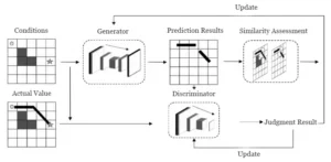
Updates to the discriminator are jointly determined by its judgments of true values and predicted values.
Updates to the generator are jointly determined by the discriminator’s judgment results and similarity assessments between predicted images and actual layouts.
♦ Generator and Discriminator Architecture
The proposed network employs a discriminator that uses stacked convolutional and residual blocks.
The generator utilizes a U-shaped convolutional neural network architecture, which includes downsampling layers, residual blocks, and upsampling layers, as detailed in Figure 2.
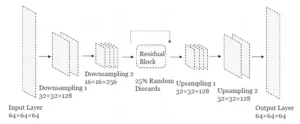
Each downsampling layer consists of a convolutional layer followed by a normalization layer.
The convolutional kernel size is 3×3 with a stride of 1, employing padding and using the ReLU activation function to adjust the output.
The normalization layer standardizes each channel using mean and variance, preventing data distribution shifts, thereby enhancing training stability and accelerating convergence.
Nine residual blocks connect the downsampling and upsampling layers. Each residual block performs convolutions with residual connections while maintaining the same number of feature channels.
A 25% random dropout is applied to prevent overfitting and further process the input features.
The upsampling layer restores the image dimensions through a transposed convolutional layer followed by a normalization layer to output the prediction results.
Network Training Evaluation Metrics
The adversarial optimization between the generator and discriminator is central to training conditional generative adversarial networks (CGANs).
The loss function in CGANs comprises two parts: generator loss and discriminator loss.
During training, we minimize the generator loss to ensure the generator’s predictions align closely with the actual wiring results.
This encourages the discriminator to classify these predictions as genuine.
Simultaneously, the discriminator loss must be maximized—enabling the discriminator to correctly identify the actual wiring as genuine while flagging the generator’s predictions as false.
The classic GAN loss function is expressed as follows:
-300x66.jpg)
Where x represents data from the dataset, z denotes data sampled from random noise, G is the generator, and D is the discriminator.
♦ Loss Function Evolution in Improved CGANs
The improved conditional generative adversarial network abandons random noise input, relying solely on labels as the basis for generation.
The generator outputs a binary classification: grid points with higher predicted values become wiring points, while those with lower values remain blank.
Using y as the input label, the loss function further evolves to:
-300x71.jpg)
Wiring problems often contain unrouted blank areas, which differ significantly from traditional image generation tasks in terms of data balance.
As a result, using the loss function of classical conditional generative adversarial networks (GANs) tends to produce all-zero outputs.
♦ Hybrid Generator Loss Structure
To address this, the improved network adopts a hybrid loss function with a wire-length penalty for the generator.
Mean Squared Error (MSE) is one of the commonly used loss functions in regression tasks.
It assigns higher penalty weights to larger error terms, measuring the squared difference between model predictions and actual values to facilitate rapid network convergence. Its mathematical expression is:
-300x72.jpg)
Where n denotes the number of elements in the prediction set; targeti represents the true value of the i-th element in the ground truth data; predi denotes the predicted value of the i-th element in the prediction set.
Binary Cross-Entropy (BCE) loss is employed to measure the discrepancy between model predictions and true values in binary classification tasks.
Since the true values in wiring tasks are logical 1s, its mathematical expression is:

Among these, pred represents the prediction result generated by the generator based on input features, while D(pred) denotes the discriminator’s judgment value on the generator’s prediction result.
♦ Wire-Length Penalty and Total Loss Formulation
Wire Length Loss (WLL) is an additional loss designed for the physical characteristics of routing tasks.
It statistically predicts the total number of points judged as wiring points in the generated routing results versus the total number of actual wiring points in the real routing results.
The generator is penalized based on the difference between these two values to prevent generating all-zero results. Its mathematical expression is:

The former represents the actual path bus length, while the latter denotes the predicted path bus length.
The generator’s total loss is the weighted sum of MSE loss, BCE loss, and WLL loss, ensuring compliance with network training requirements and physical constraints of the routing problem.
Experimental Design and Results Analysis
PCB Routing Dataset Generation
Machine learning methods require learning routing strategies from large training samples.
Since no universal PCB routing dataset currently exists across the research community, this study employs a self-built dataset as experimental data.
It comprises 10,000 64×64 three-channel PCB routing images.
In the designed routing dataset, each routing image comprises a pair of pins, obstacles along the routing path, and obstacle-avoidance connections between pins.
Pins, obstacles, and routing results are generated across three distinct channels. Obstacle-avoidance connections are generated using an improved A* algorithm.
Since PCB routing typically restricts traces to horizontal, vertical, and 45° diagonal directions with corner angles limited to 135°, the heuristic function of the A* algorithm is adjusted as follows:

Among these, g(x) calculates the actual cost from the starting point to the current routing position x, while h(x) calculates the estimated cost from the current routing position x to the endpoint.
Both utilize Manhattan distance.
C(x) imposes an additional penalty on wavy routing by evaluating the coordinates of consecutive routing points. This prevents the generation of non-linear routing paths.
O(x) avoids obstacles in the routing path by adding extra loss for each obstacle encountered.
Experimental Environment and Evaluation Metrics
The experiment was conducted on a platform equipped with an Intel Core i7-12700KF CPU and an NVIDIA RTX 3060 GPU.
For parameter management, the Adam optimizer was employed to uniformly control parameters.
Its first-order moment estimation decay rate was set to 0.9, the learning rate to 0.0001, and the batch size to 16.
Performance evaluation metrics included error degree, line length ratio, and generation time.
Error degree measured the percentage difference between predicted and actual images to validate generation validity.
Line length ratio assessed accuracy by comparing generated routing to original routing grid counts.
Generation time measured total task completion time versus traditional algorithms to evaluate routing speed differences.
Analysis of Experimental Results
The model was trained using a self-built dataset, with 80% allocated as the training set and 20% as the test set. The specific experimental workflow is illustrated in Figure 3.

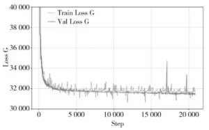
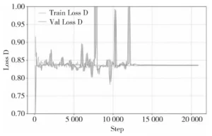
Figure 4 shows the loss variation of the generator during training, while Figure 5 displays the loss variation of the discriminator during training.
The gray dashed line represents the model’s loss during training, and the black solid line indicates the loss validated on the test set after each training iteration.
Training converged after approximately 5,000 batches and reached its final performance after 10,000 batches.
Both generator and discriminator losses exhibited significant fluctuations during training but ultimately converged to expected values.
The validation results mirrored the training outcomes, demonstrating the model’s ability to effectively learn wiring patterns.
♦ Performance Comparison Across Multiple Models
Table 1 presents the average performance metrics of the proposed generative network on the test set.
For comparison, it includes common neural network models such as Diffusion Models, Multilayer Perceptrons (MLP), Variational Autoencoders (VAE), and classical generative adversarial models.
Simultaneously, the routing results from the A* algorithm serve as the baseline comparison, with its wire length ratio set to 1 and error ratio set to 0.
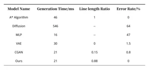
In terms of time, the routing generation model takes approximately 50% of the time required by the traditional A* algorithm, while the classic CGAN model exhibits similar processing times.
The MLP model demonstrates the shortest prediction time, whereas the Diffusion model requires the longest processing duration.
In terms of accuracy, MLP and Diffusion models struggle to converge during training, producing results with high noise levels and significant error rates, rendering their line length ratios practically meaningless.
Specifically, the MLP model consists of multiple linear layers stacked with activation functions, resulting in poor learning capabilities.
The Diffusion model treats image processing as a denoising problem for random noise.
However, in wiring problems, a large number of pixels are blank points requiring high precision, making it difficult to train an efficient denoising pattern.
VAE models similarly map inputs to noise following a specific distribution before decoding, yielding poor prediction results.
While both VAE and classic CGAN models achieve near-zero error rates, the line length ratio metric reveals that VAE predictions are entirely zero values.
CGAN predictions are also predominantly zero.
The few non-zero values come from random noise points in obstacle regions or from original pins on the routing path.
As a result, CGANs are incapable of completing the routing task.
♦ Effectiveness of the Proposed Routing Generation Network
The proposed routing generation network achieves zero overall error, with a line length ratio highly close to the actual value.
Its generated routing closely resembles real routing and effectively completes the task.
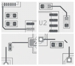
The routing results are shown in Figure 6, where black traces represent the predicted routing. The top row displays accurate generation results, while the bottom row shows suboptimal generation with breakpoints.
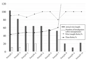
To further evaluate the routing effectiveness, Figure 7 presents the number of breakpoints, line length ratio, and the ratio of generation time to A* search time for test samples with varying line lengths.
The white bar charts represent the number of breakpoints, displayed at 10 times magnification for clarity.
Experimental results indicate that the proposed routing method shows significant advantages when the actual line length is long (>40).
It achieves a time overhead of approximately 50% compared to the traditional A* algorithm.
However, for shorter actual wire lengths (<20), the proposed routing method incurs higher time overhead than A*. For samples 8 to 10, the time overhead ratio exceeds 200%.
In sample 9, with an actual wire length of only 10, the A* algorithm’s smaller search space resulted in a routing time of just 2ms.
♦ Breakpoint Repair via A Post-Optimization*
The number of discontinuities in the generated results affects routing reliability.
When no breaks exist, the predicted routing network matches the A* algorithm’s results.
When breaks are present, intermittent unrouted regions appear along the correct path.
To further optimize routing outcomes, the proposed routing network is applied to practical tasks, with A* performing post-optimization on break-containing results.
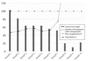
Since the generative method achieves a wire length ratio close to 90%, break-containing routing typically requires connecting only short-distance breaks.
Experiments demonstrate that the A* algorithm incurs minimal time overhead for shorter wire lengths, with optimization requiring negligible additional time.
Figure 8 illustrates the optimized generative routing results, achieving a 100% wire length ratio after eliminating breaks—matching actual routing—while only slightly increasing the time ratio.
Conclusion
This paper proposes a PCB routing generation method utilizing conditional generative adversarial networks (GANs).
By eliminating noise inputs, it avoids the impact of random noise on routing accuracy.
The network architecture is optimized to enhance feature processing capabilities, while the training evaluation function is improved to enable learning of physical characteristics in routing problems, preventing the generation of all-zero results.
Breakpoint optimization further enhances prediction accuracy.
Experiments on PCB routing datasets demonstrate that compared to traditional A* routing algorithms, the proposed method reduces average computational time by 50% while delivering accurate predictions.
This approach can assist in completing complex PCB routing tasks and reduce the computational overhead of conventional routing algorithms.
Future research may further optimize the neural network model by leveraging techniques such as large model distillation to enhance learning capabilities.
Simultaneously, expanding the routing dataset will enable broader application of this method across diverse routing scenarios.


